Table of Contents
- The Challenge
- The Architecture: A Medallion Approach
- Configuration Over Code: Generating Models from YAML
- Keeping BigQuery Costs Under Control
- Data Quality Management with Pre-Hooks and Post-Hooks
- The One-Big-Table Strategy: Pivoting for Performance
- Orchestration with Airflow
- Results & Impact
- Key Takeaways
The Challenge
Mobile games generate massive amounts of event data—player actions, in-app purchases, ad interactions, level completions, and more. For our portfolio of level-based games, we faced a complex challenge:
- Processing dozens of distinct event types across multiple games
- Creating hundreds of metrics derived from multiple events
- Tracking complex user journeys and drop-off patterns
- Keeping BigQuery costs under control
- Maintaining data quality at scale
We built a production-grade analytics pipeline using dbt that’s both powerful and cost-efficient, ultimately reducing our costs by 60% while improving performance.
The Architecture: A Medallion Approach
We adopted a three-layer architecture that balances flexibility with performance. The medallion architecture—bronze, silver, and gold layers—has become pretty much the industry standard at this point, and for good reason: it separates concerns cleanly while enabling both exploratory analysis and production-ready dashboards.

Our pipeline now processes dozens of distinct event types models handling hundreds of millions of events daily, with automated data quality checks at every layer.
Configuration Over Code: Generating Models from YAML
Writing individual SQL files for dozens of distinct event types event types meant tons of repetitive code that was a pain to maintain. Our solution: generate models from YAML configuration.
We started by creating individual SQL files for each event type. This quickly became a maintenance nightmare—inconsistent patterns everywhere, and onboarding new team members took forever because they had to learn all these slightly different implementations.
Here’s what we ended up with:
# dbt_project.yml
staging_events_config:
  events:
    - name: event_name
      params:
        param_1: string
        param_2: string
        param_3: float
      cluster_by: ["param_1", "param_2", "param_3"]
A single macro generates the complete model:
{% macro generate_event_model(event_name, event_config) %}
    {{
        config(
            materialized="incremental",
            partition_by={"field": "event_date", "data_type": "date"},
            cluster_by=["project_name"] + event_config.cluster_by,
            partition_expiration_days=90
        )
    }}

    select
        event_date,
        event_timestamp,
        user_id,
        {{ extract_event_params(event_config.params) }},
        ...
    from {{ source('firebase', 'events') }}
    where event_name = '{{ event_name }}'
        {% if is_incremental() %}
        and event_date > var('incremental_start_date')
        {% endif %}
{% endmacro %}
Now adding a new event model takes just a few lines of YAML instead of writing an entire SQL file from scratch. The time savings compound quickly as your event catalog grows.
Keeping BigQuery Costs Under Control
BigQuery costs can get out of hand fast when you’re scanning terabytes of data. Here are the strategies we used to keep spending in check.
Mandatory Partition Filters
{{
    config(
        partition_by={"field": "event_date", "data_type": "date"},
        require_partition_filter=true  -- ← Force date filters in queries
    )
}}
This one line prevents accidental full-table scans that could cost hundreds of dollars. I learned this the hard way early on.
Clustering
cluster_by=["field_1", "field_2", "field_3", "field_4"]With proper clustering, queries filtering by game and platform read about 90% less data thanks to BigQuery’s automatic pruning.
Clustering order matters a lot in BigQuery. If you have multiple games, put project_name first since you’re filtering by it constantly in dashboards and daily ETL runs. We initially tried clustering by timestamp (high cardinality) and it barely helped. Switching to low-cardinality fields first made a huge difference.
The Power of FARM_FINGERPRINT()
Our intermediate and mart layers had a ton of joins on the user_id field. Firebase generates these as random STRINGs by default, which gets expensive fast.
I came across BigQuery’s recommendation to use INT64 for joins and found this great blog post about the farm_fingerprint function. Turns out one line of code makes a big difference:
select farm_fingerprint(user_id) as user_idA few things to know about FARM_FINGERPRINT():
- Uses FarmHash Fingerprint64 with negligible collision rate for millions of users
- Returns INT64, which is way more efficient for joins and storage than STRING
- The hash is deterministic (same input always gives the same output)
- Don’t use it if you need to reverse the hash, or if you’re dealing with hundreds of millions of unique users where collision risk actually matters
This transformation cut our storage and compute costs significantly.
Data Quality Management with Pre-Hooks and Post-Hooks
dbt has these lifecycle hooks that let you run SQL before and after a model builds:
{{
    config(
        pre_hook=[""],  -- runs before model builds
        post_hook=[""]  -- runs after model builds
    )
}}
We use pre-hooks for data quality checks and post-hooks for cost optimization.
Pre-Hooks: Validating Data Before Loading
Product changes happen all the time—new games launch, event parameters get added. The YAML config needs updating, but communication between product and data teams isn’t always perfect. Sometimes the actual data looks different from what was documented.
We validate data before processing to catch these mismatches:
{{
    config(
        pre_hook=[
            "create temp table validation_results as
             select
               count(*) as total_events,
               countif(event_params is null) as null_params
             from {{ source('firebase', 'events') }}
             where event_date = current_date() - 1;

             assert (select null_params from validation_results) = 0
               as 'Found null event_params in source data';"
        ]
    )
}}
This catches schema issues before they break the pipeline.
Post-Hooks: Optimizing Incremental Loads
Standard dbt incremental models use MERGE, which scans data twice and costs more than necessary. dbt does this to create a temp table for schema comparison, which is useful, but the double scan adds up when you’re processing hundreds of gigabytes daily.
Here’s how the costs break down:
| Approach | Step 1 | Step 2 | Total |
|---|---|---|---|
| Standard dbt | Scan incremental data (100 GB) | Scan again in MERGE (20 GB) | 1.2× cost |
| Post-hook optimization | 0 (WHERE FALSE) | Single scan (100 GB) | 16.7% savings |
We found a way to keep dbt’s schema management while cutting costs:
{{
    config(
        materialized="incremental",
        post_hook=[
            "delete from {{ this }}
             where 1=1
                and event_date >= var('incremental_start_date')
                and project_name = var('project_name');
             insert into {{ this }}
             select * from {{ source('firebase', 'events') }}
             where event_date >= var('incremental_start_date');"
        ]
    )
}}

-- Main query only handles schema detection
select * from {{ source('firebase', 'events') }}
where false  -- Processes 0 bytes, only checks schema
The main query with WHERE FALSE processes zero bytes but still lets dbt compare schemas. Then the post-hook deletes only the affected partitions (cheap) and does a single INSERT instead of the double-scan MERGE. This also makes it easy to do complete data refreshes when upstream corrections happen.
We’re seeing almost 20% lower costs on incremental updates with this approach.
The One-Big-Table Strategy: Pivoting for Performance
Our Looker Studio dashboards are built so each page uses 1-2 tables. We aggregate at user granularity to get maximum flexibility for filtering and segmenting users.
User-level granularity means heavier data compared to aggregating by country or other high-level dimensions. We needed something efficient in both cost and processing time. The solution: OBT (One-Big-Table) through denormalization.
The Traditional Approach and Its Limitations
The standard way to aggregate user-level events looks like this:
select user_id, event_date, param_1,
       count(1) as event_count
from table
group by user_id, event_date, param_1
This falls apart pretty quickly. Different events need different dimensions—event_a groups by param_1 while event_b groups by param_2. You can’t join these tables because they have different granularities.
We tried a few things that didn’t work:
- Separate aggregate tables for each event type → ended up with many tables and super complex joins in Looker
- Star schema with dimension tables → join performance was terrible at user-day granularity
- Pre-aggregating to country level → lost the ability to segment users for cohort analysis
Our Solution: Pivot Before Join
Instead of grouping by dimensions, we pivot them into columns:
select
    user_id,
    event_date,
    -- Ads metrics pivoted by format
    count(case when param_1 = 'value_1' then 1 end) as num_value_1,
    count(case when param_1 = 'value_2' then 1 end) as num_value_2,
    sum(case when param_1 = 'value_3' then param_3 else 0 end) as revenue_value_3,

    -- IAP metrics pivoted by product type
    count(case when param_2 = 'value_4' then 1 end) as num_value_4,
    sum(case when param_2 = 'value_5' then param_3 else 0 end) as revenue_value_5
from events
group by user_id, event_date
We handle this SQL pattern with custom macros where the values, fields, and aggregate functions come from config files.
Why This Works So Well in BigQuery
BigQuery’s columnar storage is the secret sauce here. You might have 100 columns for different event metrics, but when your dashboard only looks at Ads data, you’re only charged for those Ads columns.
Even better, you can unpivot everything back into long format and still get the benefits:
select user_id, event_date,
    'value_1' as param_1,
    num_value_1 as event_count
union all
select user_id, event_date,
    'value_2' as param_1,
    num_value_2 as event_count
When you query with a filter:
select user_id, event_date, event_count
from view
where param_1 = 'value_1'
BigQuery only scans the num_value_1 column, not num_value_2. This is actually more cost-efficient than clustering because clustering only helps when each data block is big enough to contain just one specific value. More details in the BigQuery docs.
The tradeoff is that views are slower than materialized tables, but the cost savings and flexibility usually make it worth it.
Since everything’s denormalized, we also store user attributes (demographics, A/B test assignments) directly in the OBT. No runtime joins needed when loading dashboards.
The main benefits:
- No joins means better performance—BigQuery prefers denormalized data
- Process heavy data once in the intermediate layer, then every mart table can query it directly
- Just 2 main intermediate models power all our mart tables instead of managing dozens of normalized ones
Orchestration with Airflow

We used to run ETL manually for each game using BigQuery scheduled queries. Scheduled queries are fine for simple stuff, but they don’t handle dependencies well and backfilling is a nightmare. Since they can’t integrate with dbt, we moved to Airflow.
The Parallel Execution Challenge
One wrinkle with our setup: DAGs for different projects can’t run in parallel. We store data from all projects in a single table, so when dbt tries to create temp tables with the same name for multiple projects, things conflict.
Instead of parallel execution, we dynamically generate DAGs for all games and use Airflow’s Triggers or Dataset-Aware Scheduling to control execution order.
Making Backfills Easier
Don’t use incremental logic like this with Airflow:
where event_date > (select max(event_date) from {{ this }})It makes backfilling annoying. Use dbt variables instead:
where event_date >= var('incremental_start_date')Airflow has this super useful Jinja variable {{ ds }} that you can use as your start date to run ETL incrementally. Makes historical data loads way easier.
Results & Impact
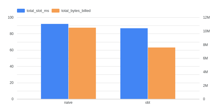
I built a small end-to-end comparison using one project and 7 days of data to show the real-world difference. Both pipelines ingested the same raw data but used different modeling approaches.
Setup:
- Same raw dataset, sample time window
- Extracted 3 representative event types from different categories
- Two pipelines: “Normal” (naive normalization) vs “OBT” (One-Big-Table denormalization)
Here’s what the architectures look like:


Performance:
- Processing hundreds of millions of events per day
- End-to-end pipeline: Under 1 hour (raw events to business dashboards)
- Incremental updates: 3-5 minutes
- Dashboard load times: 40-50% faster on full refreshes
Cost savings:
- 50% reduction in daily ETL costs vs the naive approach
- 30% lower costs on Looker Studio dashboard queries
- 60% reduction in storage costs
Developer experience:
- New event type: few lines of config vs 100+ lines of SQL
- Way fewer tables to manage
- Schema evolution for pivot columns happens automatically
- Automated data quality tests throughout
Key Takeaways
A few things I learned building this:
- Configuration beats code for repetitive stuff. The upfront investment pays off quickly.
- Partitioning and clustering aren’t optional at scale—they’re the foundation of keeping costs down.
- Generating tests from config keeps quality checks synced with your models without extra work.
- Custom incremental strategies can beat dbt’s defaults for certain use cases.
- Runtime queries in macros give you truly dynamic SQL generation.
This pipeline was built by a small data team for mobile games with millions of daily active users. All code patterns shown are production-tested and optimized for BigQuery costs.
Tech Stack: dbt • BigQuery • Airflow
Related Reading
Disclaimer: This post discusses general architectural patterns and optimization techniques for analytics. All examples have been simplified and anonymized for educational purposes. Specific implementation details, business metrics, and proprietary information have been modified or omitted to protect confidential data. The techniques described are applicable across various data engineering contexts beyond the specific use case presented.